Moral hazard arises when one party in a transaction can take actions that affect the value of the transaction for the other party. However, those actions are either unobservable or only imperfectly inferable by the affected party. This problem typically occurs in situations where two conditions are present: hidden action and risk aversion.
Hidden action: Refers to actions taken by one party that cannot be directly monitored or measured by the other party. As a result, the affected party cannot perfectly determine whether adverse outcomes are due to poor performance, lack of effort, or external factors.
Risk aversion: At least one of the parties involved must prefer avoiding risk. They value stability and predictability, often making them cautious about transactions or agreements that expose them to unpredictable outcomes.
The moral hazard problem is fundamentally about the misalignment of incentives between parties. Specifically, the party whose actions are unobservable might not have adequate incentives to act in the best interest of the other party.
Solving Moral hazard conflicts implies solving two challenges:
Provision of adequate incentives: Designing mechanisms to motivate the party taking the hidden action to behave in a way that aligns with the other party’s goals.
Efficient risk distribution: Finding a balance in how risk is shared between the parties, so that each party bears the appropriate level of risk without undermining incentives.
These two objectives often conflict. There is a substitution effect: when one party is overly shielded from risk, they may lack the incentive to take efficient actions that benefit the other party. As a result, designing an optimal compensation or incentive scheme requires balancing risk-sharing with providing the right incentives.
The focus of this class will be moral hazard conflicts arising within a firm, typically between a shareholder (the pricipal) and a manager (the agent). The principal aims to hire the agent for running a risky project, and offers the agent a contract which stablishes the agent’s compensation conditional on the outcome of the risky project. The agent first decides whether to accept the contract and then how much effort put into managing the project. The principal requires informations to infer the value of the project’s outcome and the agent’s effort to be able to compute the agent’s compensation and its own net profits.
In this setting, accounting is naturally embedded into moral hazard problems. Accounting information must have several key characteristics to be useful for decision-making. Accounting information must be relevant, comparable, verifiable, and timeliness. Scholars have studied how these characteristics can be used to design optimal contracts that mitigate moral hazard problems.
This reading note starts by developing a simple example of a moral hazard problem to illustrate the nature of the problem and the trade-offs involved in solving it. We then move on to a more general moral hazard model, allowing us to add further features to the model. We will also discuss how accounting systems must generate performance measures, and how these measures can be used to design optimal contracts. Lastly, we refer to the literature on relative performance evaluation and dynamic incentive contracts.
1.0.1 A very simple example
Let’s assume that a company (principal) hires a manager (agent) responsible for running the business. The company’s outcomes depend on both random factors and the manager’s effort. For now, let’s assume the effort can be either high (H) or low (L), and the company’s outcomes can either be success (S) or failure (F). The company’s profit in the success scenario is $360, and in the failure scenario, it is $200. The probability of success is 75% with high effort and 25% with low effort.
Therefore, the expected profit of the principal when effort is high is: 360 \times 0.75 + 200 \times 0.25 = 320. In contrast, when the effort is low the expected profit is: 360 \times 0.25 + 200 \times 0.75 = 240.
This can be summarized in the following table:
High Effort (H)
Low Effort (L)
Success (S)
75%
25%
Failure (F)
25%
75%
Expected Profit
$320
$240
We assume that the principal seeks to maximize the expected value of their net profits (expected value minus the payment to the agent). For now, let’s consider the principal to be risk-neutral.
The agent (manager) aims to maximize an expected utility function of the form:
U = U(w) - v(e)
Where U(w) is the utility of the payment received (remuneration), and v(e) is the cost of effort e.
We can distinguish four possible cases:
Observable effort, risk-neutral agent
Non-observable effort, risk-neutral agent
Observable effort, risk-averse agent
Non-observable effort, risk-averse agent
1.0.2 Observable Effort, Risk-Neutral Agent
Let’s assume an agent with a utility function U = w - v(e), and a reservation utility of \underline{U} = 81. The costs of effort are v(L) = 0 and v(H) = 63. (The numbers are arbitrary and chosen to facilitate later comparisons.)
If the principal settles for low effort, they offer the agent a salary equal to the reservation utility w = 81. The expected profit for the principal is 240, and the net benefit is 240 - 81 = 159.
If the principal wants to ensure high effort, the agent’s remuneration must cover the disutility of effort, i.e., w = 81 + 63 = 144. The net profit for the principal in this case is 320 - 144 = 176.
Thus, for the principal, the best alternative is to offer a fixed payment of 144 and obtain an expected profit of 176.
1.0.3 Non-Observable Effort, Risk-Neutral Agent
Now, consider the case where the effort is non-observable and the agent continue being risk-neutral. In this case, the conflict between incentives and risk distribution is easily resolved. The most effective way to provide incentives is to make the agent bear all the consequences of their decisions.
The contract cannot depend on effort because effort is neither observable nor verifiable. However, results such as profits are observable. Therefore, the principal can exploit the correlation between effort and profits to incentivize the agent. The principal will pay X in case of success (S), and Y in case of failure (F). This introduces uncertainty for the agent.
The principal can induce high effort by offering the agent a contract characterized by a compensation conditional on the outcome: W_E and W_F, with the following requirements:
Individual Rationality: The utility for the agent must be greater than their reservation utility.
Incentive Compatibility: The utility of exerting high effort must be greater than the utility of low effort, i.e.,E[U(A)] > E[U(B)].
As it is inefficient for the principal to pay more than needed to influence effort, the previous system of inequations are solved at the equality conditions. The optimal contract in this case involves:
w_S = 184, \quad w_F = 24.
1.0.4 Observable Effort, Risk-Averse Agent
What happens when we have a risk-averse agent? For example, assume the utility function U = w^{1/2} - v(e), where v(H) = 3 and v(L) = 0, and the reservation utility is \underline{U} = 9.
To induce low effort, it is sufficient to offer a fixed salary that yields a utility level equal to or greater than the reservation utility (w=\underline{U}^2=81). The principal’s expected net profit is 240 - 81 = 159, the same as in the scenario with a risk-neutral agent.
To induce high effort, the agent needs to be compensated for the additional disutility of the high effort. As effort can be observed, this can be achieved with a fixed salary of 144=(\underline{U}+3)^2, conditioned on high effort . Thus, the expected net profit for the principal is 320 - 144 = 176, higher than the profit for low effort (though it may not always be optimal to pay for high effort).
In this case, the agent’s risk aversion does not pose a problem since there is no uncertainty involved. The agent’s action and payment are not contingent on the state of nature.1
1.0.5 Non-Observable Effort and Risk-Averse Agent
The lack of observability of effort forces to create the compensation contract contingent on outcomes (which are correlated with effort) or abandoning variable compensation altogether. In this scenario we can see the main conflict in moral hazard problems:
Efficient Risk Distribution: the risk-neutral party (the principal) should bear all the risk, while the risk-averse party (the agent) remains on the certainty line.
Incentive Problem: For proper incentives, the agent must perceive differences in remuneration based on their effort level.
The challenge is to find the optimal balance between incentive provision and risk distribution. In the case of a risk-neutral agent, this was not a significant issue, as simply transferring residual control to the agent solved the problem. However, in this case, any variable compensation scheme must compensate the risk-averse agent for the risk they bear.
For comparison, let’s keep the utility function and parameters from the previous section. If the principal desires low effort, a fixed salary of 81 is sufficient. However, to incentive high effort, the contract with w = 144 will no longer suffice because effort is not observable, and uniform wages provide an incentive to cheat by exerting low effort.
The contract that induces high effort must meet both the individual rationality and incentive compatibility constraints, expressed as:
The second constraint can be written as 0.5[U(w_S) - U(w_F)] \geq 3. This captures the difference in utilities associated with the remuneration in each state, ensuring that high effort is chosen over low effort. The solution for this system of equation is w_E = 182.25 and w_F = 56.25. The expected cost of the contract that incentives high effor for the principal is 0.75 \times 182.25 + 0.25 \times 56.25 = 159.75, leaving them with an expected net benefit of 320 - 159.75 = 169.25.
It is important to note that inducing high effort now has a higher cost for the principal compared to the observable effort case. The cost has increased from 144 to 159.75. The additional 6.75 is the cost of non-observability, which economically corresponds to compensating the agent for the risk assumed.
2 General Model of Moral Hazard
This section borrows from Lambert (2001) Section 2 and Bolton and Dewatripont (2005) Chapter 4. We present a general version of the moral hazard problem, starting with the basic framework and then applying specific functional forms for effort and performance outcomes.
Moral hazard problems can be modeled as sequential games. In the first stage, the principal offers a contract. In the second stage, the agent decides whether to accept or reject the contract, and if accepted, chooses their level of effort. The game is solved using backward induction, where the agent’s optimal actions are determined first, and the principal designs the contract anticipating those actions.
Both the principal and the agent are assumed to have full knowledge of the game’s structure, including their respective preferences and available options. They also observe the outcome and share identical beliefs about the probability distribution governing the outcome.
2.1 Agent’s Problem
In the final stage of the game, the agent selects an effort level e, affecting the probability distribution of n possible outcomes x_i. Let p_i(e) denote the probability of outcome x_i given effort e. The agent’s utility function is defined as U(w(x_i)) - v(e), where U(w(x_i)) is the utility derived from compensation w(x_i) for outcome x_i, and v(e) represents the disutility (cost) of effort.
The agent maximizes expected utility by choosing the effort level e that satisfies:
e \in \arg\max \sum_{i=1}^n p_i(e)U(w(x_i)) - v(e)
This defines the incentive compatibility constraint (ICC), which ensures the agent has an incentive to choose the desired effort level.
Before exerting effort, the agent decides whether to participate by comparing the expected utility of the contract with their reservation utility \underline{U} (outside option):
This is the participation constraint (PC), which ensures that the agent prefers the contract over their outside option.
2.2 Principal’s Problem
In the first stage, the principal designs the contract, taking into account the agent’s optimal behavior (effort choice). The principal maximizes its expected benefit B(x_i - w(x_i)), which is based on the difference between the outcome x_i and the agent’s compensation w(x_i). The principal’s problem can be written as:
Solving the ICC in Equation 1 can be complex. However, under certain conditions, the agent’s optimal effort can be determined by the first-order condition of the ICC. Assuming the agent’s optimal effort is interior, the first-order condition is:
\sum_{i=1}^n p_i'(e)U(w(x_i)) - v'(e) = 0
This simplification is often used because it avoids solving the double maximization problem in Equation 1. However, the first-order condition is necessary but not sufficient. Since effort influences both disutility v(e) and the outcome probabilities p_i(e), the expected utility function may not be concave, meaning additional solutions (including suboptimal ones) could arise.
2.4 Optimal Compensation Terms
Using the first-order condition approach, we can formulate the Lagrangian for the principal’s problem as:
The optimal contract can be characterized by taking the derivative of the Lagrangian with respect to w(x_i) for each outcome x_i, leading to the following condition:
If \mu = 0, the solution corresponds to the first-best solution, where the agent’s actions align perfectly with the principal’s objectives. However, as demonstrated by Holmström (1979), if the principal seeks to motivate effort beyond the minimum, \mu > 0. In this case, the optimal risk-sharing depends on the sign and magnitude of \frac{p_i'(e)}{p_i(e)}.
Statistically, \frac{p_i'(e)}{p_i(e)} can be interpreted as how informative the outcome x_i is about the agent’s effort level e(Milgrom 1981). The principal rewards outcomes that are more likely when higher effort levels are exerted (p_i'(e) > 0).
Finally, the shape of the optimal contract depends on the principal’s and agent’s utility functions as well as the probability distribution of outcomes. In particular, if \frac{p_i'(e)}{p_i(e)} is increasing in the outcome, satisfying the monotone likelihood ratio condition (MLRC), the contract is likely to be monotonic in the outcome, ensuring higher outcomes correspond to higher compensations.
Linearity in the Outcome
Even if the likelihood ratio is monotonic and linear in the outcome, this would not imply that the optimal compensation is also linear in the outcome. As Equation 2 shows, the shape of the contract also depends on the preference functions of the agent and the principal.
For example, assuming the the principal is risk neutral and the agent’s has an hyperbolic absolute risk aversion (HARA) utility function, then the optimal compensation is a concave function of the outcome, as shown in Equation 3.
Thus, the optimal contract is linear in the outcome if \gamma=1 (e.g., logarithmic utility function), and concave (convex) if \gamma>1 (\gamma<1).
Limited Liability
In many instances, the optimal compensation needs to be bounded below given limited liability or wealth constraints of the agent. The problem is that Equation 2 implies penalization to the agent for bad outcomes. Therefore, the optimal compensation is often nondifferentiable and has a piecewise linear form. See Mirrlees (1974).
2.5 Accounting performance measures
Now let’s add an additional performance measure to the model to check in which conditions they reduced the welfare loss relative to the first-best solution. This will be the case if the new measure increases the agent’s incentive to exert effort or improve the risk-sharing between the principal and the agent. Be y the additional performance measure. In this case, Equation 2 becomes
Thus, the optimal contract depends on the performance metric if \frac{p_i'(x,y;e)}{p_i(x,y;e)} also depends on y. However, if x is a sufficient statistic for x and y with respect to e, then the optimal contract is independent of y. This is called Holmstrom’s informativeness condition (Holmström 1979).
Sufficient Statistic
If x=e+a_1 and y=x+a_2, where a_1 and a_2 are independent random variables, then x is a sufficient statistic for y with respect to e. In other words, y does not add any information about e that is not already contained in x.
2.5.1 Optimal Contract and Linear Aggregation
Accounting systems aggregate performance measures to reduce the complexity of reporting every individual transaction or piece of non-financial information. The aggregation arises because it would be both costly and unrealistic to report all basic transactions. In practice, accountants aggregate these performance measures linearly, typically assigning equal weights to each component. For example, total cost is the sum of each cost item, and net benefits are calculated as revenues minus expenses. These aggregated measures are often used in performance evaluations and compensation schemes.
However, the linear aggregation of performance measures with equal weights raises an important question: to what extent does contract theory support this approach? Banker and Datar (1989) provides theoretical support for the linear aggregation of performance measures but also highlights that the assumption of equal weights is rarely optimal. According to their analysis, the weights assigned to different components of a performance measure should reflect their signal-to-noise ratio (the sensitivity of the measure to effort relative to its variance). Only in cases where the signal-to-noise ratio is the same for all components can the equal weights assumption be considered optimal.
To illustrate this, consider the principal-agent framework where the principal is risk-neutral, and there are two performance metrics: x and y. We will continue considering x to be the outcome, which as an observable variable it can also play the role of a performance metric. The optimal contract is derived from Equation 4, which yields:
w^*(x,y)= W \left[ \lambda + \mu \frac{p_i'(x,y;e)}{p_i(x,y;e)} \right]
where W is the inverse of the agent’s marginal utility function. We define a new compensation function s(\pi) that depends on an aggregate performance measure\pi=\pi(x,y), where:
For many probability distributions, such as those from the exponential family, the likelihood ratio is linear in both x and y. Therefore, the optimal contract supports the linear aggregation of performance metrics in those cases.
2.5.2 Optimal Weights for Aggregation
In determining the optimal weights for these performance metrics, Banker and Datar (1989) shows that for the exponential family of distributions, when both metrics are independently distributed given the agent’s effort, the optimal weights are proportional to (1) the sensitivity of the metric to the agent’s effort and (2) the inverse of the variance of the performance metrics. Specifically, if we denote the weights as \beta_x and \beta_y, the optimal weights are given by:
This shows that the optimal weights for performance measures depend on both the sensitivity of each metric to the agent’s effort and the variance of the performance metrics. In cases where the signal-to-noise ratio differs across metrics, assigning equal weights leads to suboptimal outcomes. Therefore, a key takeaway is that optimal weighting adjusts based on the informational value of each performance measure in relation to the agent’s effort.
The relevance of variables not controlled by the agent
If the principal or other agent invest in technology or capital such as the agent’s effort is more productive or the performance metric is more sensitive to its effort, then it is optimal to introduce those variables into the contract even though are not controlled by the agent. In this case, the optimal contract adjusts the compensation to subtract the principal’s investment effect on the mean outcome or adjusts the weights of the performance metrics to reflect their new informativeness.
How the optimal contract should weights performance metrics that are correlated? In that case, Equation 6 is rewritten as
so, even if the agent does not control y (e.g., \frac{\partial E(y;e)}{\partial e}=0) then both metrics should be included in the contract with weights that reflect the correlation between them.
Thus, if the metrics are positively correlated, then their weights have opposite signs. The interpretation is that the positive correlation is driven by an exogenous common factor, and by adjusting y with a negative weight some of the noise driven by the common factor in x is removed.
3 Linear-Exponential-Normal (LEN) Moral Hazard Models
In this section, we develop a widely used model in principal-agent theory that assumes linear contracts, normally distributed performance, and exponential utility for the agent. The performance outcome is modeled as the sum of effort (in monetary terms) and noise:
x = e + \epsilon \quad \text{with} \quad \epsilon \sim N(0, \sigma^{2})
We assume that the principal is risk-neutral, meaning they are indifferent to risk and only care about the expected cost of motivating the agent. The agent, on the other hand, has constant absolute risk aversion (CARA), represented by a negative exponential utility function:
Here, \eta denotes the agent’s risk aversion, and \psi(e) represents the cost of effort.
In these models, the compensation contract follows a linear form:
w = t + sx
where t is a fixed component, and s is the performance-related component.
3.1 Agent’s Problem
Using the property of normally distributed noise, \mathbb{E}\left[e^{k\epsilon}\right] = e^{k^{2}\frac{\sigma^{2}}{2}} for any k, we derive the agent’s expected utility:
\mathbb{E}\left[u(w, e)\right] = -e^{-\eta\left[t + se - \frac{1}{2}ce^{2} - s^{2}\eta\frac{\sigma^{2}}{2}\right]}
Therefore, the Certainty Equivalent (CE) of the agent’s expected utility is:
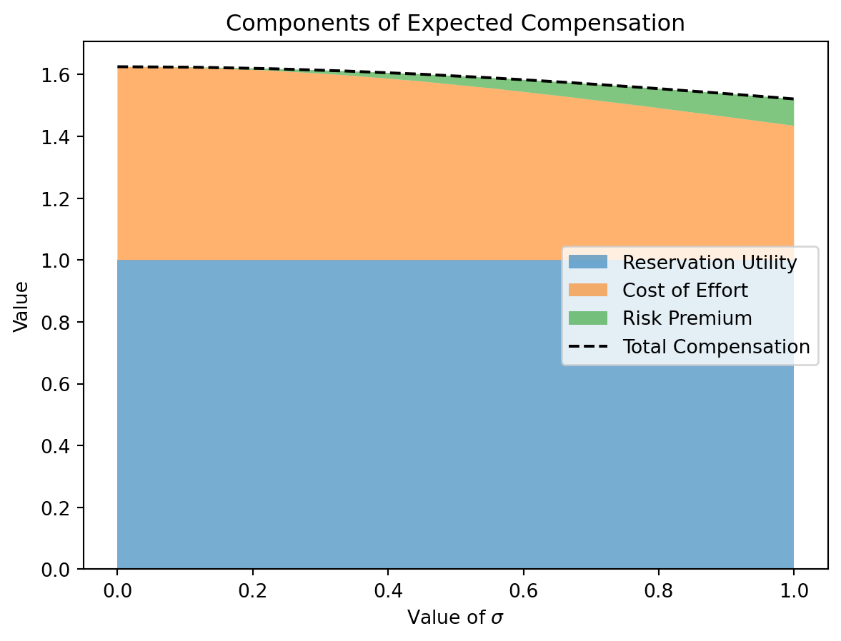
CE = \underbrace{t + se}_{\text{Expected Wage}} - \underbrace{\frac{1}{2}ce^{2}}_{\text{Cost of Effort}} - \underbrace{s^{2}\eta\frac{\sigma^{2}}{2}}_{\text{Risk Premium}}
The agent’s incentive compatibility constraint (ICC) can be reformulated as:
e \in \arg\max \hat{w}(e) = t + se - \frac{1}{2}ce^{2} - s^{2}\eta\frac{\sigma^{2}}{2}
Solving the first-order condition for effort, we obtain the optimal effort:
e^* = \frac{s}{c}
Thus, for any given incentive s, the principal can anticipate the agent’s effort level.
3.2 Principal’s Problem
The principal’s objective is to maximize their expected payoff, which is the performance outcome minus the agent’s compensation. The principal’s optimization problem is written as:
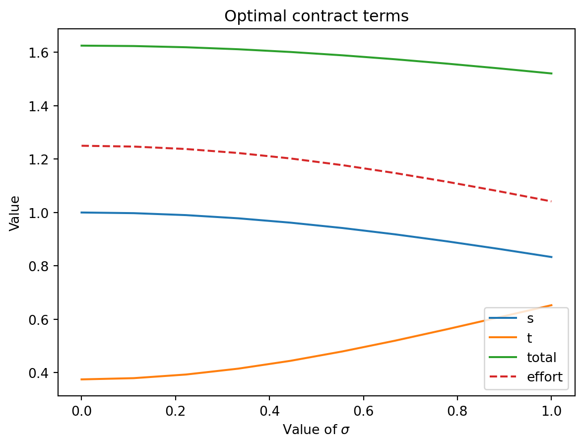
The results indicate that the variable compensation (s^*) (performance-related incentive) is higher when:
The cost of effortc is low,
The agent’s degree of risk aversion\eta is low,
The variance of the performance measure \sigma^{2} is low.
The following graphs shows the comparative statics of the optimal contract terms and utilities for different values of \sigma.
Code
import matplotlib.pyplot as pltimport numpy as npc=0.8# cost of efforteta=0.25# risk aversionw=1# reservation utility# Plot s,t,and total, for different values of sigma sigma = np.linspace(0,1,10)s =1/(1+c*eta*sigma**2)t = w - (1-c*eta*sigma**2)/(2*c*(1+c*eta*sigma**2)**2) effort = s/c total = t + s * effort plt.plot(sigma, s, label='s')plt.plot(sigma, t, label='t')plt.plot(sigma, total, label='total')plt.plot(sigma, effort, label='effort', linestyle='dashed')plt.legend()# render sigma symbol in the x labelplt.xlabel('Value of $\sigma$')plt.ylabel('Value')plt.title('Optimal contract terms')plt.show()
We can also decompose the expected compensation into its components: reservation utility, cost of effort, and risk premium.
Code
# Decomposition of the expected compensationcost_of_effort =0.5* c * effort**2risk_premium =0.5* eta * s**2* sigma**2reservation_utility = np.full_like(sigma, w)plt.stackplot(sigma, reservation_utility, cost_of_effort, risk_premium, labels=['Reservation Utility', 'Cost of Effort', 'Risk Premium'], alpha=0.6)plt.plot(sigma, total, label='Total Compensation', color='black', linestyle='--')plt.legend(loc='center right')plt.xlabel('Value of $\sigma$')plt.ylabel('Value')plt.title('Components of Expected Compensation')plt.show()
Code
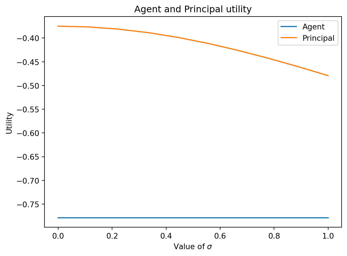
# plot the utility of the agent and principal for different values of sigmau_agent =-np.exp(-eta*(t+s*effort-0.5*c*effort**2-s**2*eta*sigma**2/2)) u_principal = effort-t-s*effortplt.plot(sigma, u_agent, label='Agent')plt.plot(sigma, u_principal, label='Principal')plt.legend()plt.xlabel('Value of $\sigma$')plt.ylabel('Utility')plt.title('Agent and Principal utility')plt.show()
3.4 Accounting Perfomance Measures
As in Section 2.5, assume that x is the outcome and y is an additional performance measure, such that:
x = e + \epsilon_x \quad \text{and} \quad y = 2e + \epsilon_y
where \epsilon_x and \epsilon_y are jointly normally distributed with zero means. The joint distribution function f(x, y; e) is a bivariate normal distribution with the following properties:
Mean vector:
\mu_{x, y} = \left(\begin{array}{c} e \\ 2e \end{array}\right)
where \sigma_x^2 is the variance of \epsilon_x, \sigma_y^2 is the variance of \epsilon_y, and \rho is the correlation coefficient between \epsilon_x and \epsilon_y.
Notice that the additional metric y is, on average, more sensitive to the agent’s effort than the outcome x, since:
This situation can arise in scenarios such as a merchandising company, where x represents net profits, but the agent has limited control over the cost of goods sold (e.g., limited negotiation power with suppliers), while the agent’s effort directly influences sales y.
3.4.1 Aggregation of Performance Measures
The accounting system aggregates both metrics x and y into a single performance measure \pi = \pi(x, y), which is used to determine the optimal compensation terms w(\pi). The relative weights for x and y, derived from Equation 7, are given by:
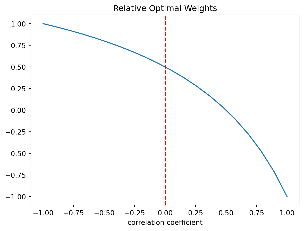
Let’s see the comparative statics of the optimal weights for different values of \rho and \sigma_y. First, let’s assume that both metrics have the same noise, \sigma_x=\sigma_y=1.25.
Code
# plot the beta_x/beta_y for different values of rho rho = np.linspace(-1,1,20)sigma_y =1.25sigma_x =1.25# subplot for rhobeta_rho = (1-2*(rho*sigma_x*sigma_y)/(sigma_y)**2)/(sigma_x**2)*(sigma_y**2)/(2-(rho*sigma_x*sigma_y)/(sigma_x)**2)plt.plot(rho, beta_rho)plt.xlabel('correlation coefficient')# add vertical line in x=0plt.axvline(x=0, color='r', linestyle='--')## add subtitleplt.title('Relative Optimal Weights')plt.show()
so, if \rho=0, the optimal weight for x is half of the weight for y, as this second signal is more sensitive to effort and has the same noise. If \rho=-1, then both both signal have full positive weight in the contract. If \rho=1, then the signals are substracted from each other in the contract to remove the common noise.
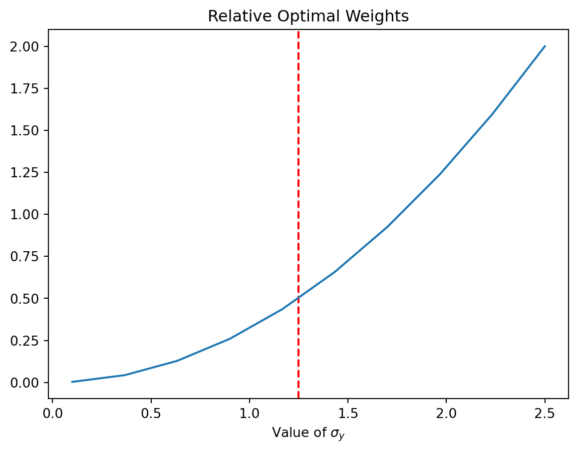
Now, let’s see the comparative statics for different values of \sigma_y, considering \rho=0 and \sigma_x=1.25.
Code
# plot the beta_x/beta_y for different values of sigma_yrho=0sigma_y = np.linspace(0.1,2.5,10)sigma_x =1.25# plot for sigma_ybeta_sigma_y = (1-2*(rho*sigma_x*sigma_y)/(sigma_y)**2)/(sigma_x**2)*(sigma_y**2)/(2-(rho*sigma_x*sigma_y)/(sigma_x)**2)plt.axvline(x=1.25, color='r', linestyle='--')plt.plot(sigma_y, beta_sigma_y)plt.xlabel('Value of $\sigma_y$')plt.title('Relative Optimal Weights')plt.show()
Here the red line despicts the same situation than in the previous plot, meaning that when both signals have the same noise. The optimal weight for x is half of the weight for y. If \sigma_y gets closer to zero, then the weight for x decreases as y gets a better relative signal-to-noise ratio.
3.5 Optimal Contract with additional Performance Measures
To evaluate how the optimal contract changes with the use of the aggregate performance metric we should compute the aggregated signal \pi(x,y)=\beta_x x+ \beta_y y using Equation 5. For simplicity, assume \rho=0.
\pi(x,y)=\frac{\sigma_y^2}{\sigma_x^2+\sigma_y^2} x+ 2 \frac{\sigma_x^2}{\sigma_x^2+\sigma_y^2} y
Now, the compensation functions depens on the aggregated signal \pi (rather than on the output x), meaning that now w(\pi)=t+s\pi. Notice that \pi \sim N(\mu_{\pi},\sigma_{\pi}^2), with
Again, for any given performance incentive s, the principal can infer the optimal effort of the agent. Relative to our initial result (e^*=s/c), Equation 9 shows that having the aggregated metric \pi in the contract increases the optimal effort level for any given value of performance incentive s as much as the sensitivity of expected value of \pi to the agent’s effort is higher than one.
The updated principal’s problem is
\begin{align*}
\underset{t, s}{\max} \quad & \mathbb{E}[x(e^*) - t - s \cdot x(e^*)] \\
\text{subject to:} \quad & t + s \cdot e^* - \frac{1}{2} c (e^*)^2 - s^2 \eta \frac{\sigma_{\pi}^2(e^*)}{2} = \overline{w}
\end{align*}
Obtaining
s^* = \frac{\frac{\partial \mu_{\pi}(e)}{\partial e}}{\left(\frac{\partial \mu_{\pi}(e)}{\partial e}\right)^2+c n \sigma_{\pi}^2} =\frac{\frac{\sigma_y^2 + 4\sigma_x^2}{\sigma_x^2 + \sigma_y^2}}{\left( \frac{\sigma_y^2 + 4\sigma_x^2}{\sigma_x^2 + \sigma_y^2} \right)^2 + c n \sigma_{\pi}^2}
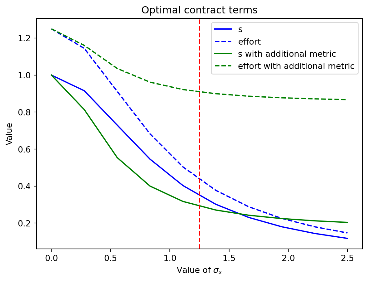
The next figure compares the optimal effort and compensation terms for different values of \sigma_x with our previous result for the case without the additional metric.
Code
c=0.8# cost of efforteta=1.5# risk aversionw=1# reservation utility# initial contractsigma_x = np.linspace(0,2.5,10)s_old =1/(1+c*eta*sigma_x**2)t_old = w - (1-c*eta*sigma_x**2)/(2*c*(1+c*eta*sigma_x**2)**2) effort_old = s_old/c # new contractsigma_y =1.25sigma_pi2= (sigma_x**2*sigma_y**2)/((sigma_x**2+sigma_y**2)**2)*(sigma_y**2+4*sigma_x**2)pi_sensitivity = (sigma_y**2+4*sigma_x**2)/(sigma_x**2+sigma_y**2)s_new= pi_sensitivity/(pi_sensitivity**2+c*eta*sigma_pi2)effort_new= (s_new/c)*pi_sensitivityplt.plot(sigma_x, s_old, label='s', linestyle='solid',color='blue')plt.plot(sigma_x, effort_old, label='effort', linestyle='dashed' ,color='blue')plt.plot(sigma_x, s_new, label='s with additional metric', linestyle='solid',color='green')plt.plot(sigma_x, effort_new, label='effort with additional metric', linestyle='dashed', color='green')plt.axvline(x=1.25, color='r', linestyle='--')plt.legend()# render sigma symbol in the x labelplt.xlabel('Value of $\sigma_x$')plt.ylabel('Value')plt.title('Optimal contract terms')plt.show()
We see that the introduction of the additional metric y leads to two effects. First, the optimal effort increases regardless of how noisy is the outcome. Second, performance-related incentive s is lower than the original case for low values of outcome volatility, but is larger when this volatility is high. This is because for low outcome volatility, the new metric is more sensitive to the agent’s effort than the output x alone, being more efficient to motivate the agent. However, for high outcome volatility, the new metric is less sensitive to the agent’s effort, so the principal needs to increase the incentive to motivate the agent.
Banker, Rajiv D., and Srikant M. Datar. 1989. “Sensitivity, Precision, and Linear Aggregation of Signals for Performance Evaluation.”Journal of Accounting Research 27 (1): 21–39. http://www.jstor.org/stable/2491205.
Bolton, Patrick, and M. Dewatripont. 2005. Contract Theory. Cambridge, Mass: MIT Press.
Milgrom, Paul R. 1981. “Good News and Bad News: Representation Theorems and Applications.”The Bell Journal of Economics 12 (2): 380–91. http://www.jstor.org/stable/3003562.